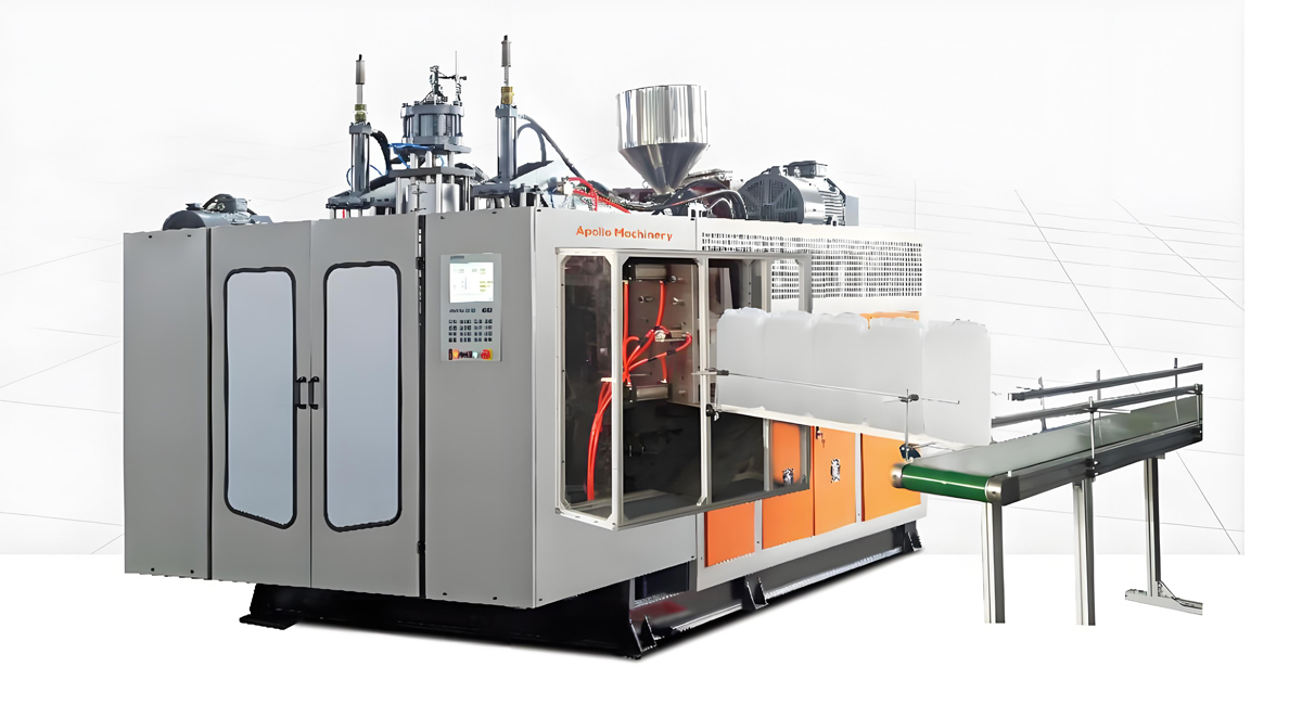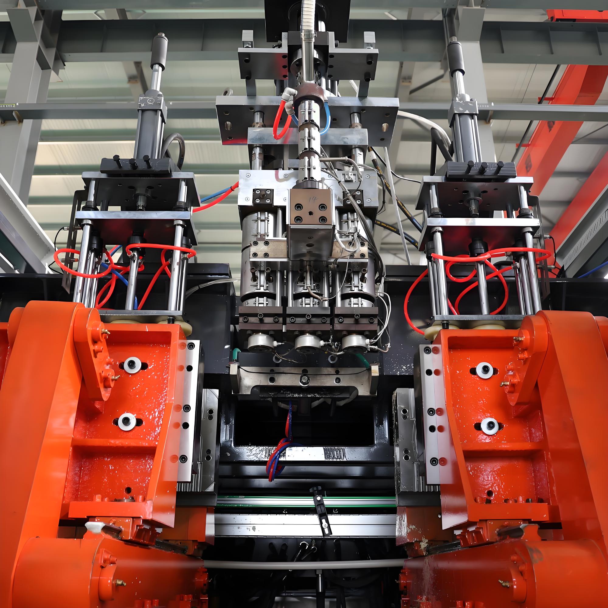

ROI calculation for an extrusion blow molding machine is fundamentally a question about the revenue side of the equation, not the purchase order. Two buyers can install identical extrusion blow molding (EBM) lines in the same month, feed them the same HDPE blow molding grade, and end up with payback horizons that differ by a factor of three. The difference is never the machine badge. It is the combination of shift pattern, changeover discipline, good-part yield, cavity architecture, gram weight control and order-book saturation that determines how quickly the asset converts itself back into working capital.
This guide builds a complete, index-based investment model for extrusion blow molding equipment. Every figure in this article is expressed as a dimensionless index, a multiple, a percentage, a month count or a physical engineering parameter such as kWh/kg or pcs/h. No currency values appear anywhere, because absolute figures vary by region, resin contract, labor market and tariff regime, and because the structural relationships between the levers are far more useful to an investment committee than a point estimate that expires in a quarter. We set a reference configuration at 100 index points and measure everything against it.
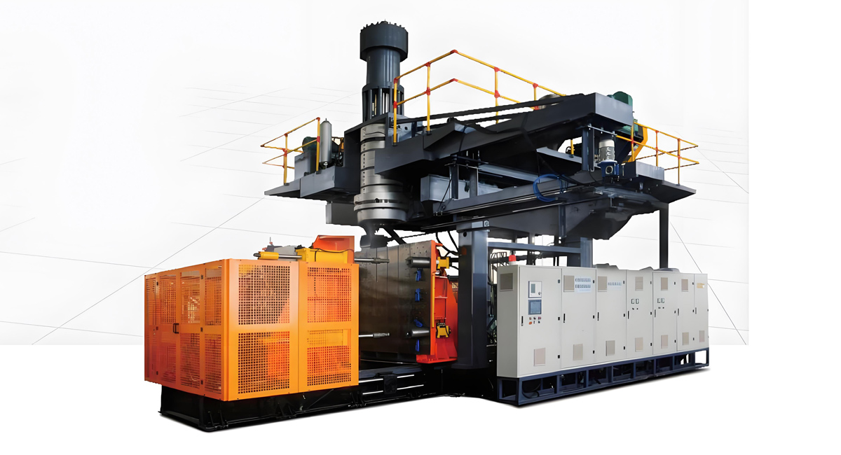
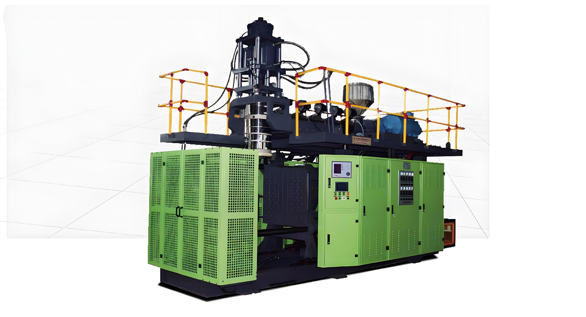
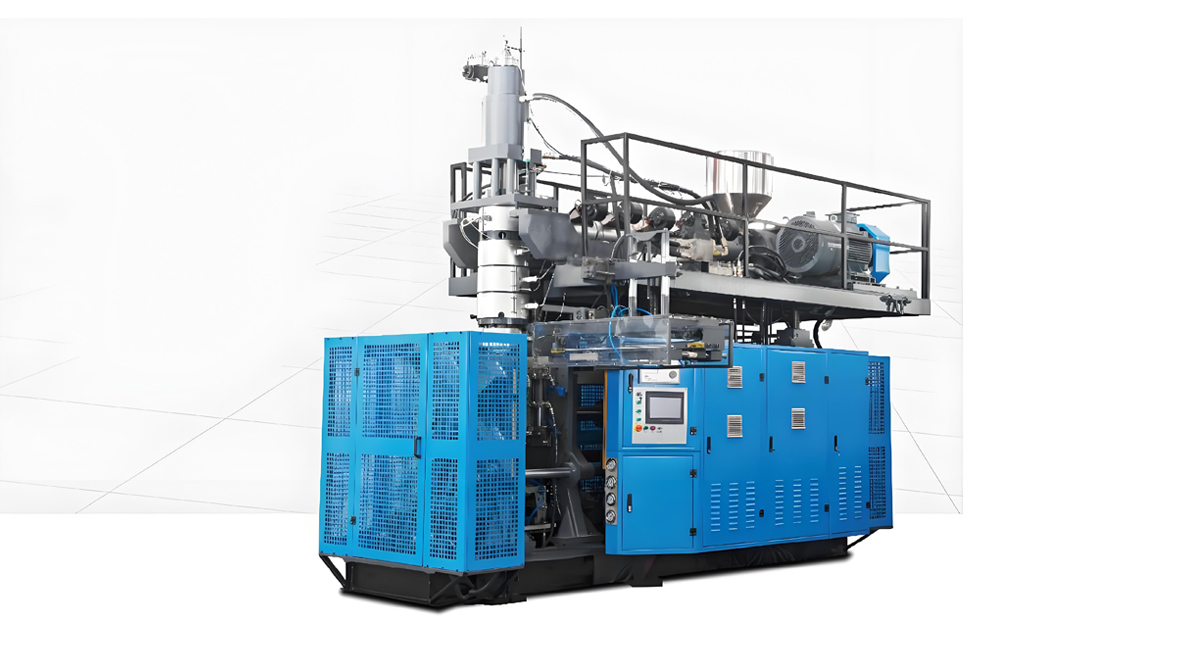
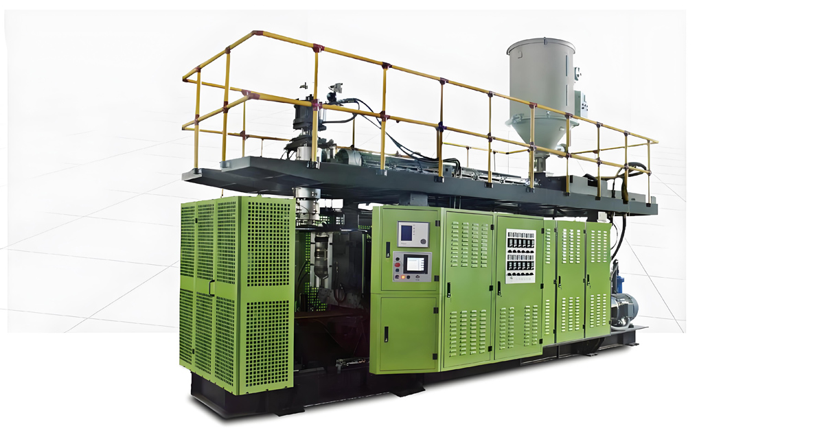
Apollo, a Wanplas factory based in Zhangjiagang near Shanghai, has spent more than twenty years building automatic extrusion blow molding machines across ten series and over eighty models, with more than 4,000 sets running in over 90 countries. That installed base spans the entire product spectrum discussed here: ABLB series machines for containers from 200ML to 20L, ABLD series machines for large-volume containers from 20L to 1500L, and a Fully Electric series covering 200ML to 20L for buyers with strict energy and cleanroom requirements. The payback patterns described in this article are drawn from how those machine classes actually behave in production, not from a spreadsheet abstraction.
By the end you will be able to construct a defensible payback model, stress-test it against a utilization-by-yield sensitivity matrix, and identify which two or three levers on your specific project deserve engineering attention before the purchase decision is finalized. Buyers running this exercise in 2026 face a particularly wide spread of outcomes, because the gap between a poorly loaded conventional hydraulic line and a well-loaded servo or fully electric line has never been larger.
Why EBM Return on Investment Behaves Differently From Generic Capital Budgeting
Extrusion blow molding is a continuous-extrusion, discrete-output process, and that hybrid character makes its investment arithmetic distinct from both injection molding and pure extrusion. The extruder and die head run continuously, producing a parison at a steady mass flow rate measured in kg/h; the clamping unit and molds convert that continuous parison into discrete containers counted in pcs/h. Any ROI model that ignores one of those two units of measure will misprice the asset.
Three structural traits separate EBM from generic capital budgeting exercises.
First, the resin stream is the dominant variable input, and it is directly programmable. In most container programs, resin accounts for the largest share of conversion economics by a wide margin. Unlike energy or labor, resin consumption per part is not a fixed property of the machine — it is set by the parison wall thickness distribution program. A 3% reduction in gram weight achieved through a 100-point parison wall thickness distribution system (PWDS) flows straight to contribution margin on every single part, forever. Very few capital equipment categories offer a software-side lever with that leverage.
Second, output is mold-bound rather than machine-bound. The extruder may be capable of 120 kg/h, but if the mold set installed today is a single cavity for a 5L jerrycan, the line will deliver a fraction of its theoretical mass throughput. Utilization in EBM is therefore a two-layer question: how many hours is the machine scheduled, and how well matched is the mold set to the extruder capacity during those hours. Buyers who evaluate only the first layer systematically overstate ROI.
Third, changeover frequency varies by two orders of magnitude across segments. A daily-chemical bottle producer serving twenty brand owners may change molds several times per week. A dedicated 200L L-ring drum plant supplying one chemical major may run the same mold for months. The same machine, the same operators and the same resin can produce completely different payback profiles purely because of changeover cadence. This is why the SMED discussion later in this article is not a lean-manufacturing footnote but a first-order financial lever.
A fourth, softer factor deserves mention: EBM assets have long economic lives. Well-maintained machines from Apollo and comparable manufacturers such as Bekum and Jomar routinely remain in service well beyond a decade. That long tail means net present value and internal rate of return, which capture the full life of the cash flow stream, tell a materially different story than payback period alone, which truncates the analysis at the recovery point and ignores everything after it.
The Five Metrics That Matter: ROI, Payback, Discounted Payback, IRR and NPV
A credible extrusion blow molding machine investment case uses at least three metrics in combination, because each one is blind to something the others capture. Simple ROI ignores timing. Payback period ignores everything after recovery. IRR misbehaves when cash flows change sign. NPV is sensitive to the discount rate assumption. Used together, they triangulate.
The following table defines each metric in plain engineering language, states what it captures, exposes its blind spot, and gives a target band appropriate to EBM equipment. All values are dimensionless or expressed in months, in line with the index convention used throughout this article.
Table 1: Investment Metrics for EBM Equipment, Defined and Bounded
| Metric | Definition in Plain Terms | What It Captures | Blind Spot | Healthy Band for EBM |
|---|---|---|---|---|
| Simple ROI | Annual net gain divided by total invested capital, expressed as a percentage | Headline efficiency of capital deployment | Completely ignores when cash arrives | 35% to 75% annualized on a well-loaded line |
| Simple Payback Period | Months of undiscounted net cash inflow required to equal invested capital | Liquidity risk and financing exposure | Ignores all cash flow after recovery point | 16 to 36 months, segment dependent |
| Discounted Payback | Same as above, but each month’s inflow is discounted to present value first | True cost of capital during the recovery window | Still truncates the analysis at recovery | Typically 1.15x to 1.35x the simple payback |
| IRR | The discount rate at which the project’s net present value equals zero | Comparability against alternative uses of capital | Unstable with irregular or sign-changing flows | Should exceed the hurdle rate by a clear margin |
| NPV Index | Present value of all lifetime net inflows minus invested capital, indexed to a baseline case at 100 | Total value created across the full asset life | Highly sensitive to discount rate and horizon | Positive over a 7 to 10 year horizon at a conservative rate |
| Profitability Index | Present value of inflows divided by invested capital, expressed as a multiple | Capital efficiency when budget is rationed | Says nothing about absolute scale of the gain | Above 1.6x on a properly loaded EBM project |
How to Use the Index Convention Correctly
Throughout this article the reference configuration is defined as follows: an ABLB-class extrusion blow molding machine producing 1L HDPE daily-chemical bottles, four cavities, servo-hydraulic drive, double shift at 16 hours per day, 85% availability, 97% first-pass yield, and a conventional four-hour mold changeover performed twice per month. That configuration is assigned a payback index of 100. A payback index of 70 means the payback period is 30% shorter than the reference. A payback index of 145 means it takes 45% longer. This lets you compare configurations honestly without pretending to know your resin contract or your regional labor rate.
Modeling rule of thumb: if two of your three headline metrics disagree about whether the project is attractive, the disagreement is almost always caused by an unrealistic utilization assumption in year one. Ramp-up is real. Model the first six to nine months at 55% to 70% of steady-state output, not at nameplate.
Building the Revenue Side: Shift Pattern, Cycle Time and Yield
The revenue side of an EBM investment case rests on exactly three multiplicative factors: how many hours the machine is loaded, how many good parts it makes per loaded hour, and what contribution each good part carries. Get the first two right and the third takes care of itself; get the first two wrong and no amount of commercial optimism will rescue the model.
Annual Loading Hours by Shift Pattern
Shift pattern is the single largest determinant of payback because capital charges are fixed while output scales almost linearly with running hours. A machine scheduled 8 hours per day across roughly 250 working days offers about 2,000 scheduled hours per year. Double shift at 16 hours gives roughly 4,000 hours. Three-shift continuous operation, allowing for planned maintenance windows and statutory holidays, realistically delivers 6,000 to 7,200 hours rather than the theoretical 8,760.
Scheduled hours are not loading hours. Apply an availability factor for planned maintenance, mold changeovers, resin changes, and unplanned stoppages before you compute output.
Table 2: Shift Pattern, Loading Hours and Payback Index
| Shift Pattern | Scheduled Hours / Year | Effective Hours at 85% Availability | Annual Output Index | Payback Index (lower is faster) | Practical Notes |
|---|---|---|---|---|---|
| Single shift, 8 h/day | ~2,000 | ~1,700 | 50 | 195 | Daily thermal cycling of the die head wastes 30 to 60 min at every start |
| Double shift, 16 h/day | ~4,000 | ~3,400 | 100 | 100 (reference) | Best balance of labor cost, thermal stability and maintenance access |
| Three shift, 24 h/day | ~6,600 | ~5,600 | 165 | 64 | Requires disciplined preventive maintenance slotting and night-shift QC |
| Three shift with weekend running | ~7,800 | ~6,400 | 188 | 57 | Only justified with a genuinely saturated order book and spare parts on site |
Note the shape of that payback index column. Going from single to double shift cuts the payback index nearly in half. Going from double to triple cuts it by a further 36%. The marginal benefit is decreasing, which is exactly what an investment committee needs to see before authorizing a third shift with its associated night premium and supervision overhead.
Cycle Time: Where the Seconds Actually Go
Cycle time in extrusion blow molding is the sum of parison extrusion or accumulator discharge, mold closing, blow pin entry and inflation, cooling, mold opening, part ejection and deflashing transfer. Cooling dominates, typically consuming 55% to 70% of the total cycle on HDPE containers because heat must be removed through the wall by conduction into the mold and then into the cooling water circuit.
Because cooling scales roughly with the square of wall thickness, gram weight reduction delivers a double benefit: less resin per part and a shorter cycle. A 5% wall thickness reduction achieved without compromising top-load strength or drop performance can shave a measurable fraction off cycle time as well as material consumption. That coupling is one of the most under-modeled effects in EBM ROI analysis.
Practical cycle-time levers worth quantifying in the model include mold cooling channel design and conformal water circuits, chilled water temperature setpoint and flow turbulence, blow air pressure and internal cooling or air exchange, parison temperature profile along the barrel and die head zones, and the mechanical speed of the clamping unit and carriage.
Yield: The Multiplier That Punishes Twice
First-pass yield deserves special attention because it penalizes the model in two directions simultaneously. Every rejected container consumed resin, energy, cooling water and a full cycle slot. Unless the reject stream is granulated and reintroduced, the loss is total. With an in-house granulator feeding regrind back at a controlled ratio, the loss is reduced to the energy and cycle-slot component but never eliminated.
The gap between 92% and 98% yield is not a 6% output difference. Because rejects also consume capacity, the effective payback index difference between those two yield levels on an otherwise identical line is typically in the range of 12 to 18 index points. Common EBM reject causes with direct financial weight include uneven wall thickness distribution, pinch-off weld line weakness, parison curl or sag on large parts, contamination and black specks from degraded material in the die head, and dimensional drift after mold temperature excursions.
EBM Machine Spectrum and Hourly Output: 1L Bottles to 200L L-Ring Drums
Output rate is the bridge between machine specification and financial model, and it varies by nearly two orders of magnitude across the extrusion blow molding spectrum. A four-cavity small-bottle machine and a single-station L-ring drum machine are both extrusion blow molding machines, but they occupy completely different points on the capital intensity and revenue-per-hour plane.
The table below maps the practical output bands across the container classes that Apollo’s ABLB series (200ML to 20L) and ABLD series (20L to 1500L) cover. Part weights are typical HDPE values and will shift with resin selection, top-load specification and whether the container is certified for dangerous goods transport.
Table 3: EBM Product Classes, Output Rates and Payback Characteristics
| Product Class | Typical Cavities | Output (pcs/h) | Part Weight | Cycle Time | Capital Intensity Index | Typical Payback Band |
|---|---|---|---|---|---|---|
| 200ML to 1L daily-chemical bottle | 4 to 8 (multi-die head) | 1,800 to 3,000 | 18 to 60 g | 8 to 14 s | Medium | 16 to 24 months at double shift |
| 1L to 5L household and lubricant bottle | 2 to 6 | 1,200 to 2,200 | 45 to 220 g | 12 to 22 s | Medium | 18 to 28 months at double shift |
| 10L to 30L jerrycan and chemical pail | 1 to 2 | 60 to 150 | 400 to 1,200 g | 28 to 60 s | Medium to High | 20 to 32 months at double shift |
| 50L to 120L drum and tank | 1 | 40 to 70 | 2.5 to 6 kg | 50 to 90 s | High | 24 to 36 months at double shift |
| 200L L-ring drum (UN grade) | 1 (accumulator head) | 30 to 45 | 8 to 11 kg | 80 to 120 s | Very High | 26 to 40 months, strongly order-book dependent |
| 500L to 1500L IBC inner and water tank | 1 (large accumulator) | 8 to 20 | 14 to 40 kg | 180 to 450 s | Premium | 30 to 48 months, niche and contract driven |
Reading the Table Financially, Not Just Technically
The instinctive reaction to Table 3 is that small bottles pay back faster. That is true on average but incomplete. Small-bottle programs are contested by many suppliers, changeover frequency is high, and margin per part is thin. Large-drum programs carry higher capital intensity and a longer payback band, but they operate in a segment with far fewer qualified suppliers, longer contracts, and a compliance moat created by UN 1H1 certification. The result is a lower revenue-per-hour volatility and a much more predictable cash flow profile.
For the 200L L-ring drum specifically, the machine architecture changes fundamentally. Continuous extrusion gives way to an accumulator head, typically in the 30 to 100 L class, which stores melt and discharges it rapidly so that parison sag is controlled on a parison weighing 8 to 11 kg. Discharge speed, accumulator plunger control and a high-resolution wall thickness distribution program are the technical determinants of whether the drum passes drop test and stacking requirements at minimum gram weight. Apollo’s ABLD series is built for exactly this class of work.
Multi-Die-Head Economics on Small Containers
On the 200ML to 1L class, the die head is the multiplier. A four-cavity head running a 10-second cycle yields 1,440 pcs/h; an eight-cavity head at the same cycle yields 2,880 pcs/h. Machine hourly overhead barely changes. This is why multi-cavity small-bottle lines show the shortest payback bands in the table. The engineering caveat is that parison-to-parison weight variation must be held tight across all cavities, which requires an individually adjustable die gap or a properly balanced flow distribution in the head.
The Mold Changeover Lever: From Four Hours to Forty-Five Minutes With SMED
Changeover time is the most underestimated financial lever in extrusion blow molding, and it is also the cheapest to improve. Reducing a mold change from four hours to forty-five minutes does not require a new machine. It requires standardized tooling interfaces, staged preparation and disciplined work sequencing.
SMED — Single-Minute Exchange of Dies — is the methodology. Its core insight is that changeover tasks fall into two categories: internal tasks that can only be performed while the machine is stopped, and external tasks that can be performed while the machine is still running the previous job. Most plants perform 60% to 80% of their changeover work as internal tasks purely out of habit. Converting those tasks to external work is where the hours disappear.
Table 4: SMED Applied to EBM Mold Changeover
| Changeover Task | Conventional Time | After SMED | Technique Applied | Task Class |
|---|---|---|---|---|
| Locate mold, tools and fixtures | 25 to 40 min | 0 min | Pre-staged mold cart with shadow-board tooling kit | Converted to external |
| Cool down and purge die head | 40 to 60 min | 10 to 15 min | Purge compound scheduled into tail of previous run | Partly external |
| Unbolt and remove old mold halves | 45 to 60 min | 8 to 12 min | Hydraulic or magnetic quick clamps replacing bolt patterns | Internal, streamlined |
| Install new mold and align | 50 to 70 min | 10 to 15 min | Standardized mold base height and locating dowels | Internal, streamlined |
| Connect cooling water and blow air | 20 to 30 min | 3 to 5 min | Multi-coupling quick-connect manifold, single action | Internal, streamlined |
| Reload wall thickness profile and process recipe | 15 to 25 min | 1 to 2 min | Stored PWDS profile recalled from HMI recipe management | Internal, digitized |
| Trial shots and first-article approval | 30 to 50 min | 8 to 12 min | Pre-heated mold, known-good recipe, inline gram weight check | Internal, streamlined |
| Total | Around 4 h | Around 45 min | Roughly 80% reduction | — |
Translating Changeover Minutes Into Payback Months
The financial arithmetic is straightforward once the changeover cadence is known. Consider a daily-chemical bottle plant performing 150 mold changes per year. At four hours each, changeover consumes 600 hours annually. At forty-five minutes each, it consumes 112 hours. The 488 recovered hours represent roughly 14% of the 3,400 effective hours available on a double shift, and because those hours carry no additional capital charge, they translate almost entirely into incremental contribution.
Expressed in the index convention, a plant that moves from four-hour to forty-five-minute changeovers at that cadence typically improves its payback index from 100 to somewhere between 84 and 88. On a job-shop line running 300 changes per year the effect is roughly twice as strong. On a dedicated 200L drum line running four changes per year the effect is negligible, which is precisely why SMED investment should be scaled to changeover frequency rather than applied uniformly.
There is a second, less obvious benefit. When changeover becomes cheap, economic batch size falls. A plant that can change molds in forty-five minutes can profitably accept shorter runs, which widens the addressable order book and raises utilization. This feedback loop is why changeover reduction often outperforms its direct arithmetic in practice.
OEE Decomposition and the Non-Linear Payback Curve
Overall Equipment Effectiveness decomposes production performance into three multiplicative factors — Availability, Performance and Quality — and it is the single most useful diagnostic frame for an EBM payback model because it tells you which of the three deserves engineering attention.
- Availability = actual running time divided by scheduled time. Losses come from mold changeovers, resin changes, breakdowns, die head cleaning and waiting for materials or operators.
- Performance = actual output divided by theoretical output at nameplate cycle time. Losses come from slow cycles, reduced extruder speed to control parison sag, and micro-stoppages at the deflashing or take-out station.
- Quality = good parts divided by total parts produced. Losses come from wall thickness defects, pinch-off failures, contamination and startup scrap.
The critical financial insight is that OEE and payback period are related non-linearly. Fixed costs — capital charge, facility, supervision, minimum staffing — are absorbed first. Below the breakeven loading point, essentially all output goes toward covering fixed overhead. Above it, each additional good part contributes at a much higher rate. The payback curve is therefore steep at low OEE and progressively flatter at high OEE.
Table 5: OEE Scenarios and Their Payback Consequences
| Scenario | Availability | Performance | Quality | OEE | Good Output Index | Payback Index |
|---|---|---|---|---|---|---|
| Struggling line, frequent changeovers, weak QC | 68% | 80% | 90% | 49% | 62 | 210 |
| Typical unoptimized plant | 78% | 86% | 94% | 63% | 80 | 138 |
| Reference configuration | 85% | 92% | 97% | 76% | 100 | 100 |
| Well-run plant with SMED and inline QC | 91% | 95% | 98.5% | 85% | 112 | 86 |
| Dedicated long-run line, world class | 94% | 97% | 99.2% | 90% | 119 | 80 |
Read the payback index column from bottom to top. Lifting OEE from 49% to 63% — a 14-point gain — cuts the payback index by 72 points. Lifting it from 76% to 90% — the same 14-point gain — cuts the payback index by only 20 points. That asymmetry is the single most important structural fact in EBM investment analysis, and it has a clear practical implication: if your existing line runs below 60% OEE, fixing it will almost always outperform buying a second machine.
Diagnosing Which OEE Factor to Attack First
A simple triage rule works well in EBM plants. If Availability is below 80%, changeover and die head cleaning are the culprits and SMED plus purge discipline is the answer. If Performance is below 88%, look at parison sag forcing reduced extruder output, at cooling capacity limiting cycle time, and at micro-stoppages in the deflashing and take-out chain. If Quality is below 95%, the wall thickness distribution program, the pinch-off geometry and the mold temperature control loop are the first three places to look.
Single-Cavity Versus Multi-Cavity: The Unit Cost Index
Cavity count is the clearest example of a decision where higher capital intensity produces a faster payback, and understanding the shape of the curve prevents both under-investment and over-specification.
When cavity count increases, output per cycle rises proportionally while the hourly overhead of the machine — capital charge, operator, floor space, control system — rises only marginally. The extruder must supply more melt, so a larger barrel and drive may be required, and the die head becomes more complex. But the conversion cost per container falls steeply from one to four cavities and then begins to flatten.
Table 6: Cavity Count Versus Unit Conversion Cost Index
| Cavities | Output Multiple | Unit Conversion Cost Index | Mold Capital Index | Changeover Complexity | Best Fit |
|---|---|---|---|---|---|
| 1 cavity | 1.0x | 100 | 100 | Low | Large containers, short runs, frequent SKU change |
| 2 cavities | 2.0x | 62 | 165 | Low to Medium | Mid-volume 1L to 5L programs |
| 4 cavities | 4.0x | 42 | 290 | Medium | High-volume daily-chemical bottles, stable SKUs |
| 6 cavities | 5.8x | 36 | 420 | Medium to High | Contract packers with committed annual volumes |
| 8 cavities | 7.4x | 33 | 560 | High | Very high volume small bottles, single dedicated SKU |
Note that the output multiple falls short of the cavity count at six and eight cavities. That shortfall is real and comes from flow balance limitations in wide multi-die heads, marginally longer mold close and open strokes on a wider clamping unit, and increased deflashing load at the take-out station. Modeling a linear output multiple at eight cavities is one of the most common errors in EBM business cases.
The Hidden Constraint: Wall Thickness Uniformity Across Cavities
Multi-cavity extrusion blow molding is only economically superior if every cavity produces a container within specification. Parison-to-parison weight variation across an eight-cavity head is a genuine engineering challenge. Individual die gap adjustment, symmetric melt distribution channels and thermal uniformity across the head width are the countermeasures. Where those are not properly executed, plants compensate by running all cavities at the gram weight required by the heaviest-walled cavity, which quietly destroys the material savings that justified the multi-cavity investment in the first place.
For this reason, the decision between four and six cavities should be made jointly with the mold and die head supplier rather than as a pure capacity calculation. Apollo’s machine customization service covers exactly this scope, matching mold configuration and die head design to the specific container geometry and the buyer’s voltage and layout requirements.
Drive Technology and the Specific Energy Index
Drive technology influences payback through a single measurable quantity: specific energy consumption, expressed in kWh per kg of processed resin. Across the extrusion blow molding population, that figure spans roughly 0.35 to 0.55 kWh/kg depending on drive architecture, machine size, resin and ambient conditions.
Table 7: Drive Architecture and Energy Performance
| Drive Architecture | Specific Energy (kWh/kg) | Energy Index | Capital Intensity | Repeatability | Payback Contribution |
|---|---|---|---|---|---|
| Conventional hydraulic, fixed pump | 0.50 to 0.55 | 100 | Low | Moderate, drifts with oil temperature | Baseline |
| Variable displacement pump hydraulic | 0.45 to 0.50 | 90 | Low to Medium | Good | Small but reliable improvement |
| Servo-hydraulic | 0.40 to 0.46 | 82 | Medium | High | Best all-round choice for mixed programs |
| Fully electric | 0.35 to 0.40 | 70 | Medium to High | Very High, no oil temperature drift | Strongest at high running hours |
Apollo’s Fully Electric Series covers 200ML to 20L containers and is aimed at buyers with strict environmental, cleanliness or repeatability requirements. Beyond the energy index, the elimination of hydraulic oil removes an entire contamination pathway, which matters for pharmaceutical and food-contact containers, and removes oil-related maintenance interventions from the availability calculation.
When Hydraulic Still Wins
Fully electric is not universally superior, and an honest ROI model must say so. For 200L L-ring drums and larger tanks produced on an accumulator head, the shot must be discharged rapidly to control parison sag on a parison weighing many kilograms. Hydraulic accumulator systems deliver that instantaneous power density more economically than electric equivalents. This is why Apollo’s ABLD series for 20L to 1500L containers remains hydraulically driven while the small-container Fully Electric Series serves the 200ML to 20L range.
The decision rule is straightforward. Energy savings scale with running hours and with throughput in kg/h. On a line running fewer than about 2,500 hours per year, the energy index advantage of fully electric rarely offsets its higher capital intensity within the payback window. Above 4,000 hours per year on small containers, it usually does — and the repeatability benefit, which shows up as higher Quality in the OEE calculation, often contributes more to payback than the electricity saving itself.
Ancillary Energy Loads Buyers Forget
Specific energy figures quoted by manufacturers usually cover the machine alone. The complete line also draws power for the chiller serving mold cooling, the compressor supplying blow air, the dehumidifying dryer if the resin requires it, and the conveying and granulating equipment. Blow air in particular is a substantial and frequently ignored load; recovering and reusing exhaust blow air, and specifying the correct blow pressure rather than defaulting to maximum, are two of the cheapest energy interventions available on an EBM line.
Material Levers: Blow Molding Grades, MFR and Gram Weight Control
Resin is the dominant variable input in extrusion blow molding, which makes gram weight control the highest-leverage engineering intervention available to the ROI model. A 3% reduction in part weight, sustained across every part for the life of the mold, typically outweighs the entire energy saving available from switching drive technology.
Selecting the Right Blow Molding Grade
Extrusion blow molding requires resins with high melt strength so that the parison resists sag under its own weight between extrusion and mold close. That requirement pushes blow molding grades toward the low end of the melt flow rate scale, with broad molecular weight distribution and, for demanding applications, bimodal structures that combine processability with environmental stress crack resistance.
Table 8: Blow Molding Grade Selection and Processing Windows
| Material | Typical MFR / MVR | Melt Temperature | Drying Requirement | Typical EBM Products | ROI Relevance |
|---|---|---|---|---|---|
| HDPE, small container grade | MFR 0.3 to 0.8 g/10min (190 C / 2.16 kg) | 170 to 200 C | None normally required | Daily-chemical bottles, lubricant bottles | Highest volume, most sensitive to gram weight |
| HDPE, large part grade (bimodal) | MFR 0.15 to 0.45 g/10min (190 C / 2.16 kg) | 180 to 210 C | None normally required | 20L jerrycans, 200L L-ring drums, IBC inners | Melt strength governs minimum achievable wall |
| PP, blow molding copolymer | MFR 0.3 to 1.0 g/10min (230 C / 2.16 kg) | 190 to 230 C | None normally required | Hot-fill bottles, medical containers, clarity parts | Narrower window, higher scrap risk during startup |
| PVC, blow molding compound | K value approximately 57 to 60 | 165 to 185 C | Low, but compound must be dry | Cosmetic bottles, edible oil bottles, clarity packaging | Requires low-shear screw and precise thermal control |
| PC, blow molding grade | MVR 3 to 6 cm3/10min (300 C / 1.2 kg) | 250 to 280 C | Mandatory, to below 0.02% moisture | Returnable water bottles, technical containers | Drying energy and hydrolysis risk enter the model |
| PA / multi-layer barrier structures | Grade dependent | 230 to 260 C | Mandatory | Fuel tanks, agrochemical containers, barrier packaging | Premium segment, higher margin, longer qualification |
Values shown are typical ranges and will vary by grade and supplier; always confirm against the resin datasheet before finalizing a process window.
Parison Wall Thickness Distribution: The Software Lever
A parison wall thickness distribution system controls the die gap dynamically as the parison is extruded, so that material is placed where the container needs it — thicker at the pinch-off, the shoulder and the handle transition, thinner in the straight sidewall where it contributes little to top-load performance. A 100-point PWDS divides the parison length into one hundred independently programmable segments, which is enough resolution to control complex geometries such as handled jerrycans and L-ring drums.
The financial consequence is direct and measurable. On lines upgrading from coarse or manual wall thickness control to a 100-point system with closed-loop feedback, gram weight tolerance commonly tightens from around plus or minus 1.5% to around plus or minus 0.5%. Because production must always target the upper end of the tolerance band to guarantee that the lightest part still meets specification, tightening the band allows the nominal target weight itself to be lowered. Typical net material savings fall in the 2% to 5% range depending on container complexity.
Leverage comparison: on a typical HDPE container program, a 3% reduction in gram weight delivers a larger payback improvement than reducing specific energy consumption from 0.55 to 0.40 kWh/kg. Both are worth doing, but if engineering attention is scarce, put it on the parison program first.
Regrind Strategy and the Deflashing Loop
Extrusion blow molding inherently generates flash at the pinch-off, the neck and the tail. Depending on container geometry, flash can represent 15% to 40% of the extruded mass on complex handled containers. A closed regrind loop — beside-the-press granulator, metal separation, controlled blending back into virgin resin at a validated ratio — converts what would be a material loss into a small energy cost. Where regrind quality or color consistency is a concern, or where volumes justify it, Wanplas’s Kerke factory supplies single-screw and twin-screw extruders for pelletizing scrap into a uniform, dosable feedstock, and Wanplas’s Polyretec factory supplies washing and pelletizing lines for post-industrial and post-consumer streams.
Regrind handling belongs in the ROI model explicitly. A plant that recovers and reuses 95% of its flash has a fundamentally different material cost index than one that sells flash as scrap, and the gap widens as container complexity and flash ratio increase.
Risk Variables That Stretch the Payback Horizon
Every payback model is a forecast, and forecasts fail in predictable ways. The purpose of this section is to name the failure modes so they can be priced into the case as scenario adjustments rather than discovered later as surprises.
Table 9: Risk Register for EBM Investment
| Risk Variable | Mechanism | Direction of Payback Impact | Severity | Mitigation |
|---|---|---|---|---|
| Order book saturation shortfall | Machine scheduled for double shift but loaded for one and a half | Lengthens, strongly | Very High | Secure anchor contract before commissioning; design for SKU flexibility |
| Resin price volatility | Input cost moves faster than container pricing can be renegotiated | Lengthens during upswings | High | Index-linked pricing clauses; gram weight reduction as structural hedge |
| Exchange rate movement | Imported equipment and spares priced in one currency, revenue in another | Either direction | Medium | Match currency of financing to currency of revenue where possible |
| Tariff and trade policy change | Landed equipment cost or export market access shifts mid-project | Usually lengthens | Medium | Confirm incoterms and duty classification early; diversify target markets |
| Technology iteration | Newer machines reset the competitive cost floor before payback completes | Lengthens indirectly via price pressure | Medium | Specify upgradeable control platform and retrofittable PWDS |
| After-sales downtime | Waiting for parts or engineers destroys Availability | Lengthens | High | On-site critical spares kit; remote diagnostics; supplier with regional presence |
| Operator skill gap | Parison program never optimized beyond commissioning settings | Lengthens quietly | High | Structured training at commissioning; recipe management discipline |
| Regulatory change in target packaging market | Recycled content mandates or design-for-recycling rules alter specification | Either direction | Medium | Validate machine for regrind and PCR blends at purchase, not later |
How to Price Risk Into the Model Without Guessing
The cleanest approach is scenario weighting rather than a single risk-adjusted discount rate. Build three cases — conservative, base and stretch — differing only in utilization, yield and gram weight assumptions, then compute payback index for each. If the conservative case still clears your hurdle, the project is robust. If only the stretch case clears it, the project is a bet on execution, and the investment committee should be told so explicitly.
The after-sales variable deserves particular emphasis for buyers importing equipment. Availability losses caused by waiting for a component are indistinguishable, financially, from a machine that was never bought. This is why Wanplas brand-level commitments — engineers on-site for installation and commissioning, an annual free spare parts allowance, warranty replacement of damaged parts, production capacity guarantees and an open factory policy for pre-shipment inspection — belong in the ROI conversation rather than being treated as commercial boilerplate.
Sensitivity Analysis: Utilization Multiplied by Yield
The two variables that dominate EBM payback are capacity utilization and first-pass yield. A two-dimensional sensitivity matrix across those variables is the most decision-useful single artifact an investment case can contain, because it shows immediately whether the project is robust or fragile.
In the matrix below, the payback index is normalized so that 70% utilization combined with 97% yield equals 100. Lower numbers mean faster recovery. Utilization here means effective loading hours as a fraction of the double-shift reference of approximately 3,400 hours per year, so 140% represents genuine three-shift operation.
Table 10: Payback Index Sensitivity Matrix (Utilization × First-Pass Yield)
| Utilization \ Yield | 90% | 94% | 97% | 99% |
|---|---|---|---|---|
| 40% utilization | 232 | 216 | 205 | 198 |
| 55% utilization | 168 | 156 | 148 | 143 |
| 70% utilization | 113 | 106 | 100 | 96 |
| 85% utilization | 92 | 86 | 81 | 78 |
| 100% utilization | 78 | 73 | 69 | 66 |
| 140% utilization (three shift) | 59 | 55 | 52 | 50 |
Three Conclusions the Matrix Forces
Utilization dominates yield. Moving down a single column — from 40% to 140% utilization at constant 97% yield — cuts the payback index from 205 to 52, a factor of roughly four. Moving across a single row — from 90% to 99% yield at constant utilization — improves it by only 12% to 15%. Both matter, but if you must choose where to spend management attention, fill the machine first.
Yield matters most when utilization is already high. In absolute index points the yield improvement is worth more at low utilization, but in percentage terms the effect is fairly stable. The practical significance is different: at high utilization, scrap consumes capacity you cannot replace, because there are no spare hours left to make up the shortfall. A plant running three shifts cannot simply run longer to compensate for a bad batch.
The bottom-left quadrant is the danger zone. A project modeled at 40% to 55% utilization with 90% to 94% yield carries a payback index between 156 and 232 — roughly one and a half to well over two times the reference. Projects in that quadrant are frequently approved on the assumption that utilization will improve later. Sometimes it does. The discipline is to require an explicit, dated plan for how the machine gets filled, not an assumption that it will.
Extending the Matrix With a Third Dimension
Sophisticated buyers add gram weight as a third axis. Because material is the dominant variable input, a 3% gram weight reduction shifts the entire matrix downward by roughly 6 to 10 index points at every cell, with the larger effect at higher utilization where more material passes through the machine. This is another way of seeing why a 100-point PWDS with closed-loop weight feedback is one of the few options on an extrusion blow molding machine that reliably pays for itself.
Certification as a Revenue Gate: CE, EN 422, UN 1H1 and ISO 9001
Certification does not appear as a line in most ROI spreadsheets, yet it determines which orders you are permitted to quote. In that sense, compliance is a revenue gate rather than a cost, and its correct place in the model is on the utilization side.
Table 11: Certifications and Their Commercial Effect
| Standard | Scope | What It Gates | Effect on the ROI Model |
|---|---|---|---|
| CE marking | Machinery safety conformity for the European market | Legal placement of the machine on the market in the EEA | Prerequisite; without it European utilization is zero |
| EN 422 | Specific safety requirements for blow molding machines | Guarding, interlocks, clamping unit access, control reliability | Reduces incident and stoppage risk; supports insurance and audit |
| UN 1H1 / 1H2 | Performance certification for plastic drums carrying dangerous goods | Drop, stacking, leakproofness and hydraulic pressure testing | Unlocks the chemical packaging segment with premium margin index |
| ISO 9001 | Quality management system | Supplier qualification with multinational brand owners | Raises achievable utilization by widening the qualified customer base |
| Food contact regulations | Material and article compliance for food-contact containers | Resin selection, regrind policy, colorant and additive approval | Constrains regrind ratio, which feeds back into material cost index |
| ISO 14001 | Environmental management system | Tenders from brand owners with formal sustainability criteria | Increasingly a qualification threshold rather than a differentiator |
The UN 1H1 Case in Detail
The 200L L-ring drum is the clearest example of certification-driven ROI. A drum intended to carry dangerous goods must pass a defined suite of performance tests, including drop testing on the chime at conditioned temperature, stacking under load, leakproofness and hydraulic pressure. Passing those tests at minimum gram weight is a genuine engineering achievement that depends on wall thickness distribution accuracy, pinch-off design and resin selection with adequate environmental stress crack resistance.
The commercial consequence is that the field of qualified suppliers narrows sharply. Fewer competitors, longer contracts and higher switching costs for the customer combine to produce a more stable revenue-per-hour profile than the daily-chemical bottle segment offers, even though the raw payback band in Table 3 looks longer. An investment committee comparing a small-bottle project against a drum project should weight not only the expected payback but the variance around it.
Machine Safety Features That Also Protect Availability
Safety and uptime are aligned more often than buyers expect. Light curtains and interlocked guards on the clamping unit prevent the improvised interventions that cause both injuries and unplanned stoppages. Melt pressure monitoring and die head over-temperature protection prevent degradation events that force a full purge and cleaning cycle. Specifying a machine to EN 422 and CE requirements is therefore not merely a compliance expense; it removes a category of availability loss from the OEE calculation.
A Seven-Step ROI Worksheet You Can Run Before Signing
The following sequence turns everything above into a repeatable procedure. Work through it in order, because each step constrains the next. Express every result as an index or a percentage so the model stays portable across regions and currencies.
Step 1: Define the Product Basket, Not Just the Machine
List every SKU the machine will produce in year one and year two, with volume, container size, part weight and required cavity count. If the basket contains more than five SKUs, changeover frequency will materially affect payback and you must model it explicitly.
Step 2: Compute Theoretical Output Per Hour
For each SKU: 3,600 divided by cycle time in seconds, multiplied by cavity count, gives theoretical pcs/h. Cross-check against the kg/h capacity of the extruder and die head. If mass throughput is the binding constraint rather than cycle time, the model must use the mass limit.
Step 3: Apply the Full OEE Chain
Multiply theoretical output by Availability, Performance and Quality. Be conservative in year one: a newly commissioned line rarely exceeds 70% OEE in the first quarter even with experienced operators, and ramp-up to steady state typically takes two to three quarters.
Step 4: Build the Annual Hours Model
Start from scheduled hours by shift pattern, subtract planned maintenance, subtract changeover hours calculated as frequency multiplied by duration, and subtract resin and color change purge time. The remainder is your effective loading hours.
Step 5: Quantify the Material Position
Calculate resin consumption as good parts multiplied by target gram weight, divided by the flash recovery efficiency, plus startup and changeover scrap. Then compute the same figure at the gram weight achievable with a 100-point PWDS. The difference between the two is the material lever, expressed as a percentage of total resin throughput.
Step 6: Compute All Five Metrics and the Sensitivity Matrix
Produce simple ROI, simple payback, discounted payback, IRR and NPV index for the base case, then rebuild the payback index across the utilization-by-yield matrix. Identify which cell your conservative case occupies and confirm it still clears the hurdle.
Step 7: Stress the Model Against the Risk Register
Take each row of Table 9 and ask what happens to the base case if that risk materializes at moderate severity. Any risk that pushes the payback index above your tolerance threshold requires an explicit mitigation owner and deadline before the purchase order is issued.
What Apollo Brings to the Execution Side
A payback model is only as good as the execution behind it, and most of the levers in this article are execution levers rather than specification levers. Apollo, a Wanplas factory, operates an 8,000 square meter plant in Zhangjiagang with an annual production capacity of around 100 sets, and supports buyers through the phases where payback models usually break: machine customization including mold configuration and voltage adaptation, factory inspection before shipment under the Wanplas open factory policy, engineers on-site for installation and commissioning, structured operator training, ongoing usage tracking and periodic customer visits.
The Wanplas brand-level commitments apply across all factories: an annual free spare parts allowance, free replacement of parts damaged within warranty, a transportation guarantee, a production capacity guarantee, and a quality standards guarantee under which a failure to meet agreed standards triggers a refund plus additional compensation. Those commitments map directly onto the Availability and Performance terms of the OEE equation, which is where payback is actually won or lost.
Buyers whose product basket extends beyond extrusion blow molding can source adjacent equipment within the same brand: Wanplas’s YuDa factory for PET bottle blow molding including FGX high-speed series machines, Wanplas’s Aibim factory for injection blow molding of small pharmaceutical and cosmetic containers from 3ML to 1000ML, Wanplas’s Kerke factory for twin-screw compounding and pelletizing, and Wanplas’s Polyretec factory for washing and recycling lines. Consolidating suppliers across a plant simplifies spare parts logistics and training, both of which show up in the Availability term.
Frequently Asked Questions
What is a realistic payback period for an extrusion blow molding machine?
Expressed as a range rather than an absolute figure, a well-loaded small-container line running double shifts at high yield typically recoups its investment within roughly 16 to 28 months, while large-container and 200L L-ring drum lines run longer, in the 26 to 40 month band. A single-shift line with frequent changeovers can take two to three times as long as the same machine on double shift. Utilization and yield, not the machine badge, dominate the outcome.
Which single lever shortens EBM payback the most?
Capacity utilization. Moving from single shift to double shift roughly doubles annual output against a largely fixed capital base, which compresses the payback index by nearly half. The second strongest lever is gram weight control through parison wall thickness distribution, because resin is the dominant variable input and the saving applies to every part produced for the life of the mold.
Should I use payback period or NPV to justify the purchase?
Use both, plus IRR. Payback period answers a liquidity question — how long is capital at risk — and is the right frame when financing is tight. NPV answers a value question across the full asset life, which matters because extrusion blow molding machines commonly run well beyond a decade. IRR makes the project comparable against other uses of capital. If the three metrics disagree, the disagreement usually points to an unrealistic ramp-up assumption.
Does a fully electric extrusion blow molding machine always pay back faster?
No. A fully electric machine consumes roughly 0.35 to 0.40 kWh per kg versus 0.50 to 0.55 kWh per kg for conventional hydraulic, but it carries higher capital intensity. The energy advantage only outweighs that premium when annual running hours are high, so fully electric machines pay back fastest on double or triple shift small-container production. For 200L drums on an accumulator head, hydraulic drive remains the better technical and financial choice because of the shot speed required.
How much can a 100-point parison wall thickness distribution system actually save?
On lines upgrading from coarse or manual control, gram weight tolerance typically tightens from around plus or minus 1.5% to around plus or minus 0.5%. Because production must target the top of the tolerance band to guarantee the lightest part meets specification, tightening the band allows the nominal target weight to be lowered. Net material savings usually fall in the 2% to 5% range, with the larger figures on complex handled containers.
How do I model the ramp-up period realistically?
Assume the line reaches roughly 55% to 70% of steady-state good output in the first quarter after commissioning, 75% to 85% in the second, and steady state somewhere in the third or fourth quarter. Ramp-up is driven by operator familiarity with the parison program, mold optimization and QC calibration rather than by mechanical readiness. Models that assume nameplate output from month one typically understate payback by three to six months.
Is it better to buy one large machine or two smaller ones?
Two smaller machines give redundancy, allow parallel SKUs without changeover, and reduce the consequence of a single breakdown, but they consume more floor space and more operators. One larger multi-cavity machine gives a lower unit conversion cost index but concentrates risk. As a rule, if your product basket has more than five active SKUs or if a single line stoppage would breach a customer service level agreement, two machines usually produce the better risk-adjusted payback.
How does regrind affect the ROI calculation?
Substantially. Flash can be 15% to 40% of extruded mass on complex containers. A closed regrind loop with a beside-the-press granulator, metal separation and controlled blending converts most of that from a material loss into a small energy cost. Food-contact and pharmaceutical applications constrain regrind ratios, so the achievable recovery rate must be validated against the applicable regulations before it is credited in the model.
What OEE should I assume for a new EBM line in the business case?
For a first-year base case, 70% to 76% is defensible for a well-supported installation with trained operators. Assuming 85% or higher from the start is optimistic unless the line is dedicated to a single long-running SKU. If your model only works at 85% OEE in year one, it is a fragile model and should be re-run at 70%.
How many mold changes per year justify investing in quick mold change?
As a rough threshold, above roughly 60 to 80 changeovers per year the recovered hours from a four-hour to forty-five-minute reduction become financially significant, and above 150 changeovers per year the case is compelling. Below about 20 changeovers per year — typical of dedicated drum lines — the investment is hard to justify on payback grounds alone, though standardized interfaces still reduce error risk.
Does UN 1H1 certification change the ROI picture for 200L drums?
Yes, and in a favorable direction that raw payback tables understate. UN 1H1 performance certification narrows the field of qualified suppliers, which supports longer contracts, more stable order books and a higher margin index. The raw payback band for drum lines is longer than for small bottles, but the variance around it is lower, which often makes it the better risk-adjusted investment.
What does specific energy consumption of 0.35 to 0.55 kWh per kg actually include?
It normally covers the machine itself: extruder drive, barrel and die head heating, clamping and carriage movement, and the machine’s own control system. It usually excludes the chiller serving mold cooling, the compressor supplying blow air, resin drying if required, and conveying and granulating equipment. When comparing quotations, confirm the measurement boundary, because ancillary loads can add a meaningful fraction to the total.
How should exchange rate and tariff risk be treated in the model?
Qualitatively, as scenario adjustments rather than as a single risk premium. Match the currency of financing to the currency of revenue where possible, confirm incoterms and duty classification before contract signature, and run a conservative case in which landed cost and spare parts cost move adversely. The purpose is not to forecast the movement but to confirm that the project survives it.
Can an existing hydraulic EBM machine be upgraded rather than replaced?
Often yes, and it frequently produces a better payback index than replacement. Retrofitting a modern parison wall thickness distribution controller, upgrading to a variable displacement or servo pump, adding quick mold clamps and a quick-connect cooling manifold, and installing inline gram weight monitoring together address the material, energy and availability levers without a new capital purchase. Retrofit is most attractive when the mechanical structure of the machine is sound and the limiting factor is control resolution.
Conclusion
ROI calculation for an extrusion blow molding machine is best understood as a structured argument about four numbers: how many hours the machine runs, how many good parts it makes per hour, how many grams of resin each part consumes, and how much of the theoretical output survives changeovers and defects. Everything else — drive technology, cavity count, control resolution, certification — acts through those four numbers.
The evidence in this article points to a clear hierarchy. Capacity utilization is the dominant lever, capable of moving the payback index by a factor of four across the realistic range. Gram weight control through a 100-point parison wall thickness distribution system is second, delivering 2% to 5% material savings that compound over the life of every mold. Changeover reduction from four hours to forty-five minutes is third, worth roughly 12 to 16 payback index points on a plant with frequent SKU changes. Energy efficiency, though genuinely valuable at 0.35 to 0.40 kWh/kg on fully electric machines versus 0.50 to 0.55 kWh/kg on conventional hydraulic, ranks fourth in most container programs.
The practical recommendation follows directly. Before comparing machine specifications, build the utilization-by-yield sensitivity matrix for your own product basket and find out which quadrant your project occupies. If it lands in the upper-left danger zone of low utilization and modest yield, no equipment decision will rescue it and the commercial plan needs work first. If it lands in the lower-right region, the remaining question is which configuration — cavity count, drive architecture, wall thickness control resolution — extracts the most value from an order book you already have.
Apollo, a Wanplas factory with more than twenty years in extrusion blow molding, ten machine series, over eighty models and more than 4,000 sets running in over 90 countries, builds machines across the full span discussed here: ABLB series for 200ML to 20L, ABLD series for 20L to 1500L, and the Fully Electric series for 200ML to 20L. If you are preparing an investment case, share your product basket, target shift pattern, container geometry and certification requirements, and the Apollo engineering team will help you populate the output, cycle time and energy terms of your model with figures that reflect your actual configuration rather than a generic benchmark.